Decoder-Only Transformer Architecture

Introduction
Architecture Overview
Input Tokens, Embedding, and Positional Encoding
Decoder Model
- 4.1. Masked Multi-Head Attention
- 4.2. Add & Norm
- 4.3. Feed-Forward Neural Network (FFNN)
- 4.4. Add & Norm
- 4.5. Full Decoder Block
Linear Layer
Training Pipeline
- 6.1. Flattening and Loss Computation
- 6.2. Updating Learnable Weights
- 6.3. Loss Computation During Training
Inference Pipeline
- 7.1. Input Preparation
- 7.2. Autoregressive Token Prediction
- 7.3. Iterative Process
Additionals: Vanishing gradients and regularization techniques
References

1. Introduction

The goal of this readme is to describe in details the Transformer Decoder Architecture. We will be presenting all the different layers and illustrating each step using a dummy example.

2. Architecture Overview

The Decoder only architecture contains multiple concepts, that we will see in detail. To begin, we will lay the general overview of the pipeline, mentionning all the core components.

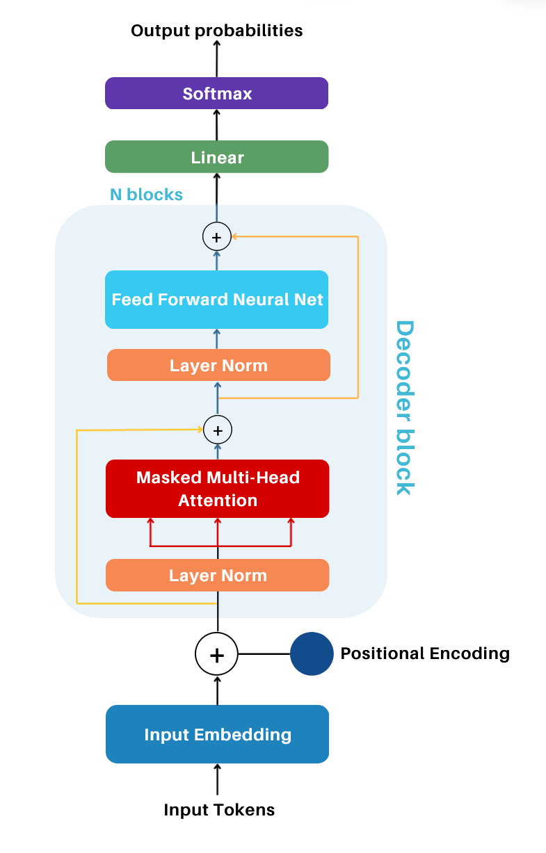
The Decoder architecture is built upon many different components, namely (and in order):

Input Tokens These represent the tokens processed by the model. During training, they are batches of input sequences from the dataset. During inference, they refer to the input text provided to the model.
Input Embeddings Tokens are mapped to dense vector rpz. using an embedding matrix, capturing semantic relationships.
Positional Encoding is added to the embeddings, enabling the model to understand the order of tokens in a sequence.
Decoder block
- Masked Multi-Head Attention Computes attention scores to capture contextual relationships between tokens. Masking ensures that the model only considers past and current tokens during training.
- Norm and Add Layer normalization first, followed by a residual connection to stabilize training and improve gradient flow.
- Feed Forward Neural Network Fully connected network with a non-linear activation for learning complex relationships.
- Add & Norm Layer normalization first, followed by a residual connection after the feed-forward network.
Linear Layer Projects the output matrix from the decoder block to a space matching the vocabulary size, producing logits.
Softmax Converts logits into probabilities, representing the likelihood of each token in the vocabulary.
Output probabilities The probabilities of tokens in the sequence generated by the model.

3. Input Tokens, Embedding, and Positional Encoding

The first step of the model begins with processing the input tokens, also called tokenization.

Input Tokens: Tokenization consists of splitting text into smaller units or tokens. There exist various strategies, such as character-level tokenization, word-level tokenization, subword tokenization (like Open AI models using with Byte Pair Encoding). This allows to create a vocabulary, containing all unique tokens which are mapped to unique IDs.
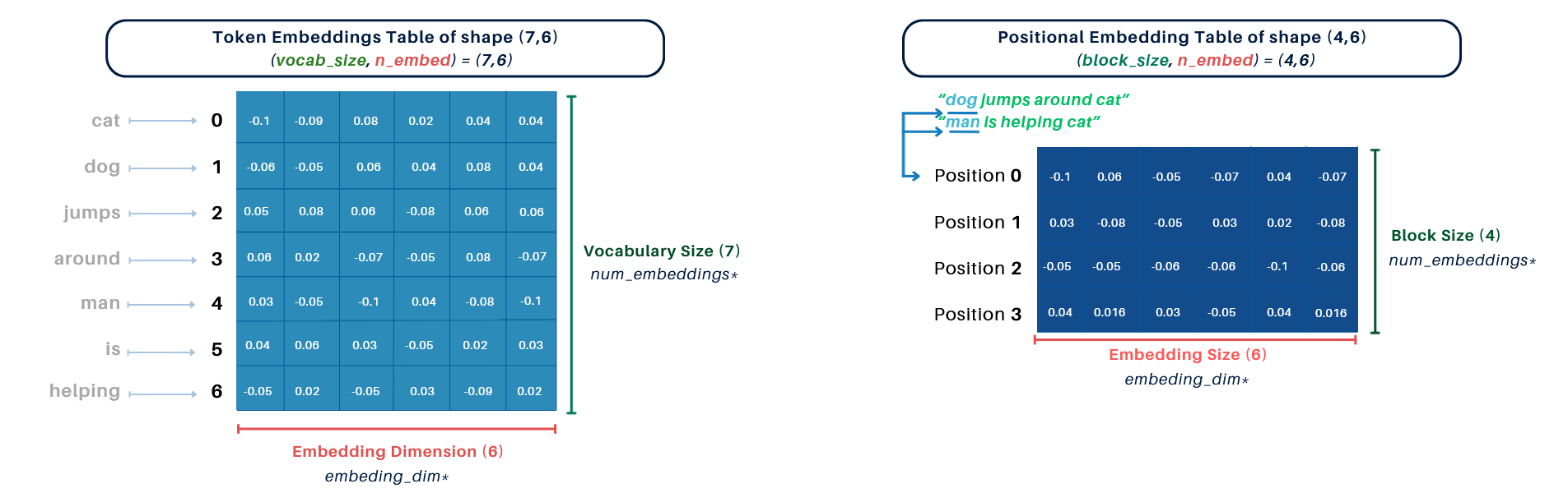
Input Embedding Matrix: The tokens are then mapped to a dense vector representation, also called the embedding matrix. This matrix is learnable and is optimized during training through backpropagation. It is of shape (vocab_size, n_embed), where vocab_size is the total number of tokens in the vocabulary and n_embed is the embedding dimension. This matrix is essential for the Decoder as it allows to capture semantic relationships between tokens.
Positional Encoding Matrix: Positional Encoding is added to the token embeddings to provide the model with information about token positions in the sequence. It is of shape (block_size, n_embed), where block_size is the sequence length and n_embed is the embedding dimension. One important note is that the positional encoding ensures that tokens at the same positions in different sequences receive the same positional embedding, as it is only based on their position within the sequence. Finally, this positional encoding, unlike the one used in the original Transformer paper, is based on learned embeddings, which is also optimized during training.
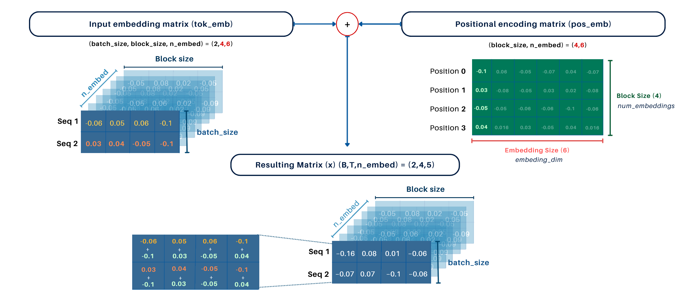
Combined Input Matrix: The Input Embedding Matrix and Positional Embedding Matrix are added together to form the input matrix for the model, allowing both semantic and positional information to be incorporated.

Example:

For the following explanation, we use this example dataset:

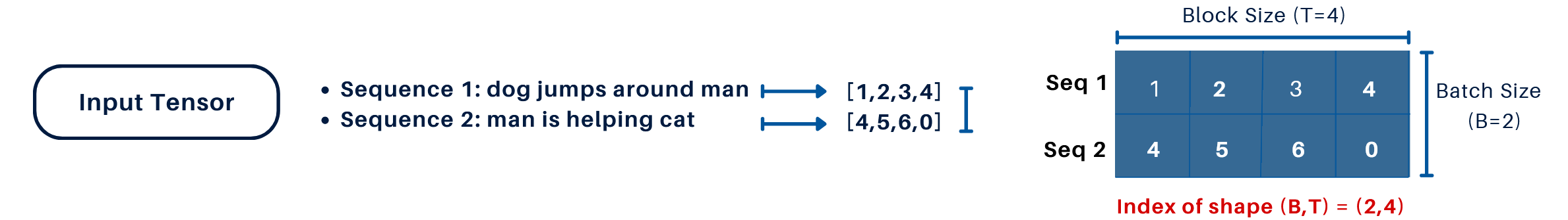
Input Dataset: "dog jumps around cat man is helping cat"
Tokenization: ["dog", "jumps", "around", "cat", "man", "is", "helping", "cat"]
Unique IDs: {"cat": 0, "dog": 1, "jumps": 2, "around": 3, "man": 4, "is": 5, "helping": 6}
Vocabulary Size (vocab_size): 7
Embedding Dimension (C): 6
Block Size (T): 4
Batch Size (B): 2

1. Input Representation:

The model's input is a tensor of shape (B, T) = (2, 4), as depicted on the image:

2. Embedding Tables:

Token Embedding Table: Shape (vocab_size, n_embed) = (7, 6)
Positional Embedding Table: Shape (block_size, n_embed) = (4, 6)

3. Embedding Process:

Input Embedding Matrix (tok_emb): Maps the input tokens (B, T) to a dense matrix of shape (B, T, C) = (2, 4, 6).
Final Input Matrix (x): The positional encoding matrix (4, 6) is added (via broadcasting) to the token embedding matrix, resulting in a final shape of (B, T, C) = (2, 4, 6).

4. Decoder:

4.1. Masked Multi-Head Attention

Multi-Head Attention consists of multiple attention "heads" each processing the input independently to capture different aspects of relationships between tokens (e.g., semantic, syntactic). Each head operates in parallel, enabling the model to simultaneously attend various parts of the input sequence. The results from all heads are concatenated and transformed into a single output. However, more heads are not always better; their effectiveness depends on the model's capacity (embedding dimensions per head) and the complexity of the task.

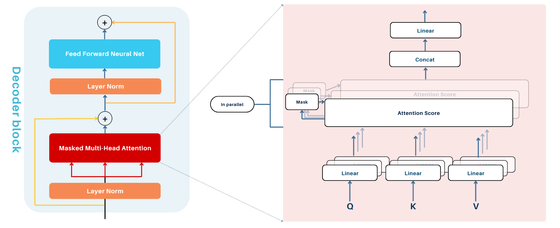
1. Key Components

Each attention head computes attention scores using three vectors derived from the input:

Query (Q): Represents the token currently being processed.
Key (K): Acts as a label for other tokens in the sequence.
Value (V): Encodes the actual information of each token.

These vectors are generated by applying separate linear transformations with learned weights:

$Q = XW_Q, \quad K = XW_K, \quad V = XW_V$

$X$ : The input embeddings of shape $(B, T,C)$
$W_Q, W_K, W_V$ : Learnable weight matrices of shapes $(C, d_k)$ , $(C, d_k)$ , and $(C, d_v)$ , respectively, used to project the input embeddings into Query, Key, and Value vectors. (in_features, out_features)

Note: In PyTorch, weight matrices like $W_Q, W_K, W_V$ are defined in the shape $(\text{out_features}, \text{in_features})$ . During computation, the transpose is applied implicitly, making the operation $Q = XW_Q$ mathematically equivalent to $Q = XW_Q^T$ , without requiring an explicit transpose.

2. Attention Score Calculation

Determines how much focus each token should have on others in the sequence using the Scaled Dot-Product Attention formula: $$ \text{Attention}(Q, K, V) = \text{softmax}\left(\frac{QK^T}{\sqrt{d_k}}\right)V $$

$QK^T$ : Computes the similarity between the Query and Key vectors (dot product).
$\sqrt{d_k}$ : A scaling factor to stabilize the attention scores where $d_k = \frac{n_{\text{embed}}}{\text{num_heads}}$ .
$\text{softmax}$ : Normalizes the attention scores into probabilities.
$V$ : Represents the values aggregated using the attention probabilities.

3. Masking in the Decoder

To ensure causal (sequential) behavior, masking is applied in the decoder:

Why Masking? During token prediction, the decoder must not "peek" at future tokens or the rest of the target sequence. Masking ensures only previous and current tokens are visible.
How Masking Works:
- A mask is applied to the attention scores before the softmax step.
- Masked positions are set to $-\infty$ , forcing their softmax values to be zero.

4. Final Output:

Each attention head produces an output of shape (B, T, d_k). Outputs from all heads are concatenated into a single matrix and passed through a linear layer to produce the final output of shape (B, T, C), where C is the model's embedding size.

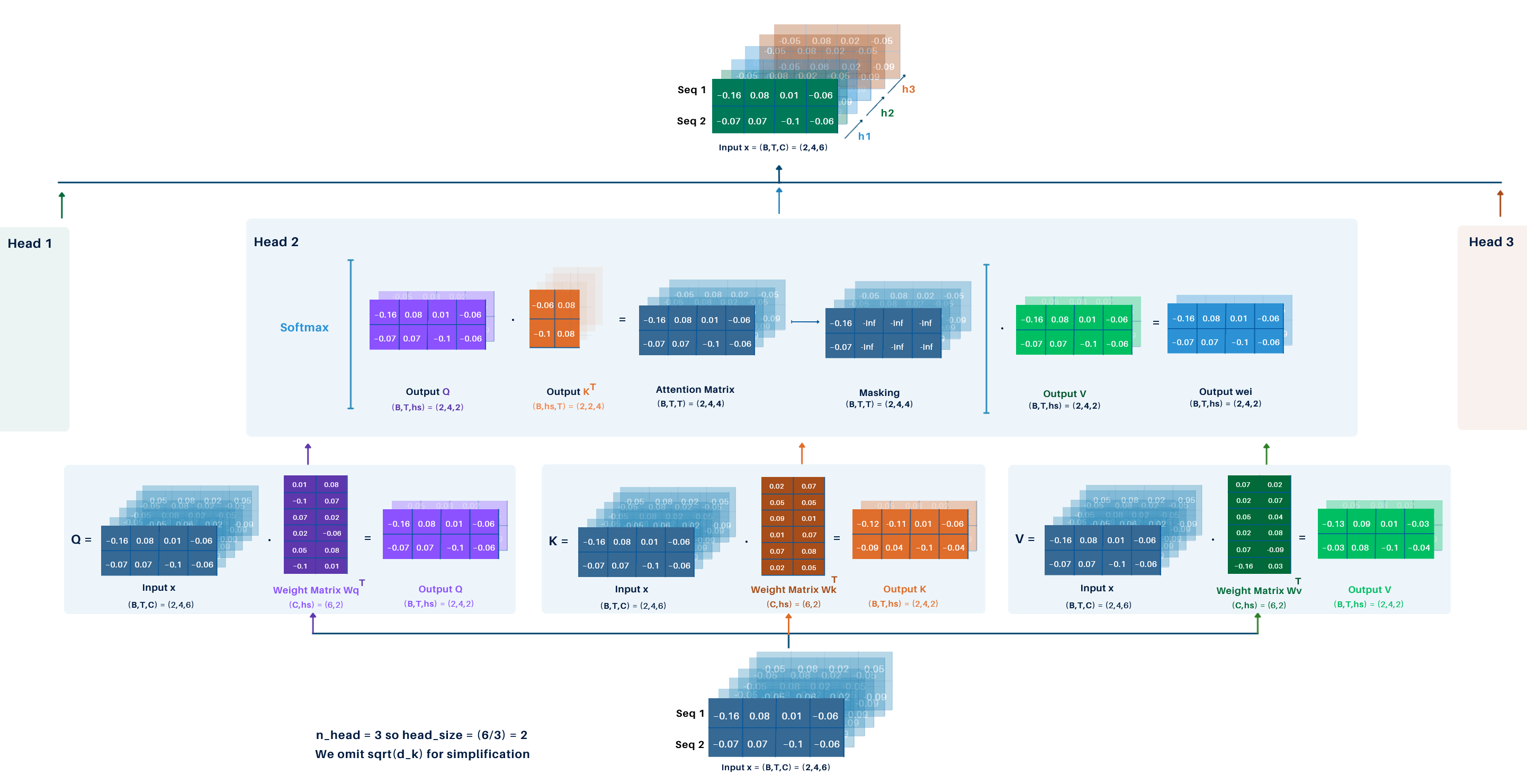
Example:

Using the previous example with the following parameters:

Batch size B = 2
Block size T = 4
Embedding dimension C = 6
Number of heads = 3

For simplicity, we omit the $\sqrt{d_k}$ scaling factor.

Step-by-Step Process:

Input Dimensions: Input embeddings have shape (B, T, C) = (2, 4, 6).
Query, Key, and Value Matrices
- Three linear transformations produce Q, K, and V.
- Each matrix has shape (B, T, h_s) = (2, 4, 2), where h_s (head size) is C divided by the number of heads: 6/3 = 2.
- Weight matrices for Q, K, and V are of shape (h_s, C).
Attention Score Computation
- Compute the dot product of Q and K^T, resulting in the attention score matrix wei of shape (B, T, T) = (2, 4, 4).
- Apply masking and softmax to normalize the scores.
Attention Output
- Multiply the attention scores with V, yielding an output matrix for each head of shape (B, T, h_s) = (2, 4, 2).
Head Concatenation
- Concatenate the outputs from all 3 heads to form a single matrix of shape (B, T, C) = (2, 4, 6).

This final matrix is the output of the masked multi-head attention layer. This is illustrated in the following image:

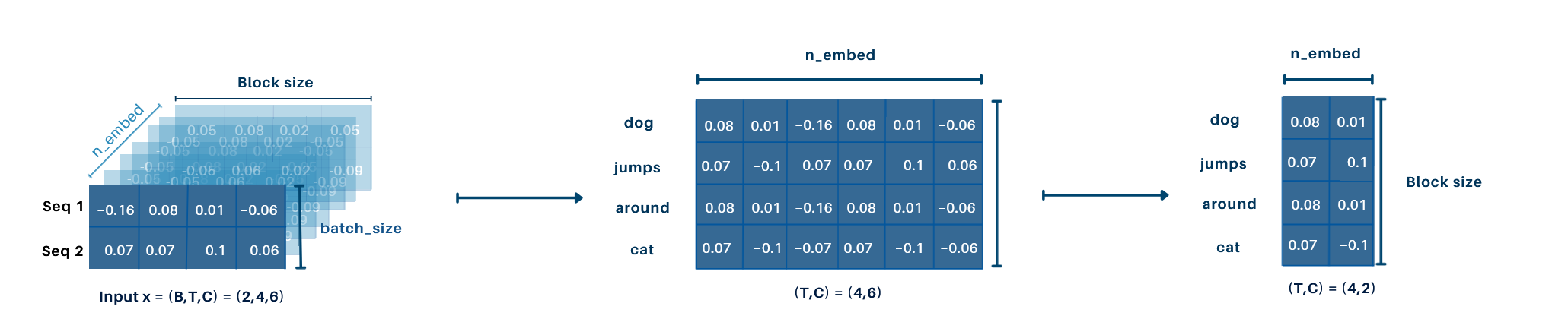
Simplified Example:

We start with the input matrix (B, T, C) = (2, 4, 6). To focus on a single sequence, we reduce it to (T, C) = (4, 6). For simplicity, we further reduce the embedding dimension to C = 2, giving (T, C) = (4, 2). The head size is set to h_s = 2.

Disclaimer: This process is applied simultaneously across all sequences in the batch, but this illustration focuses on what happens for a single sequence for clarity. In practice, it operates on all sequences independently within the batch.

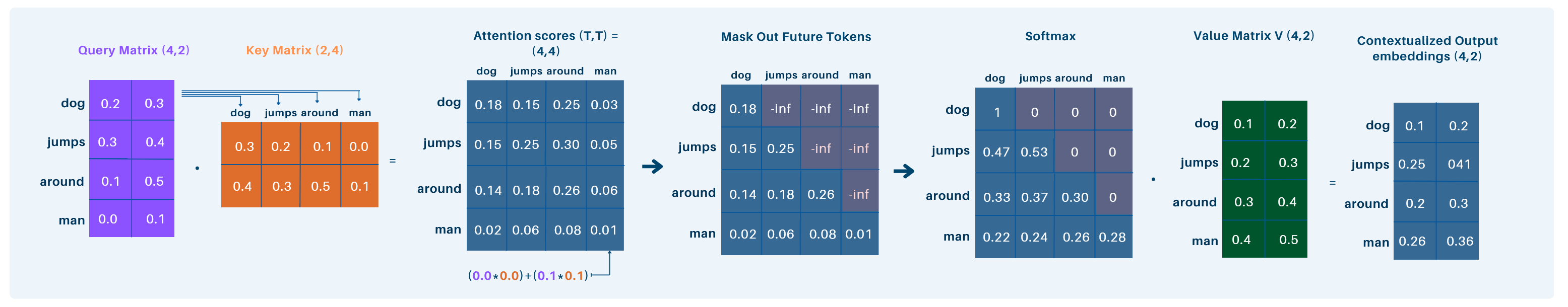
Query Matrix (Q):
- Input X: (T, C) = (4, 2), Weight W_Q: (C, h_s) = (2, 2)
- Result: Q = (T, h_s) = (4, 2)
Key Matrix (K):
- Weight W_K: (C, h_s) = (2, 2)
- Result: K = (T, h_s) = (4, 2)
Attention Scores:
- Q: (T, h_s) = (4, 2), K^T: (h_s, T) = (2, 4)
- Result: QK^T = (T, T) = (4, 4)
- Each token in the query is evaluated against all tokens in the key (which act as labels) to compute attention scores.
Softmax:
- Apply softmax to normalize QK^T, keeping the shape: (T, T) = (4, 4)
Value Matrix (V):
- Weight W_V: (C, h_s) = (2, 2)
- Result: V = (T, h_s) = (4, 2)
Contextualized Output:
- Multiply attention scores with V: (T, T) \cdot (T, h_s) = (4, 4) \cdot (4, 2)
- Result: Output = (T, h_s) = (4, 2)
- The attention scores are used to aggregate values $V$ , producing the final contextualized embeddings.

Final Output: The final contextualized embedding for the sequence has shape: (T, h_s) = (4, 2).

This process computes how much focus each token in the sequence should give to every other token, combining the values $V$ weighted by the attention scores to produce the output.

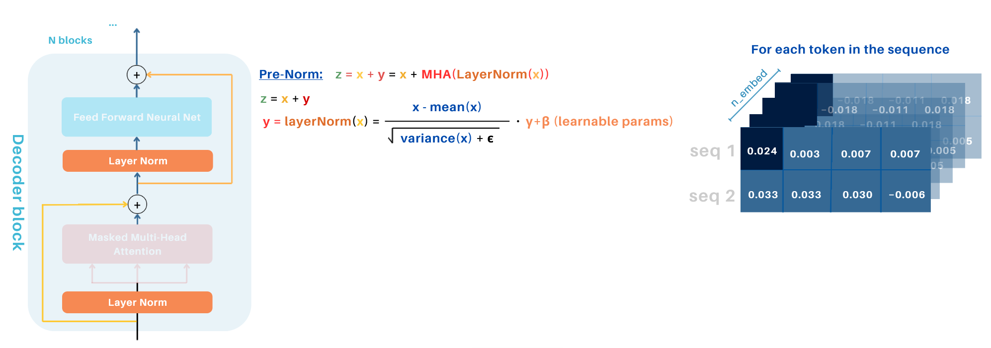
4.2. Norm & Add (Pre-norm)

Norm & Add is an essential step in the Transformer Decoder architecture, combining layer normalization and residual connections to stabilize and enhance the training process. Here, Layer Normalization is applied before the sublayer, independently to each token embedding across its feature dimensions.

Key Steps:

Layer Normalization (Norm):
- The input to the Masked Multi-Head Attention (or Feed-Forward Network in subsequent steps) is normalized first.
- This step ensures stability by normalizing the intermediate activations across the feature dimensions to have a consistent mean and variance.
Residual Connection (Add):
- The output of the sublayer (e.g., Masked Multi-Head Attention or Feed-Forward Network) is added to the input of the respective layer (e.g., input embeddings or intermediate outputs).
- This "shortcut" helps retain original input information, improves gradient flow, and mitigates issues like vanishing gradients.

Why Norm & Add?

Normalization Benefits:
- Prevents instability caused by vanishing or exploding gradients.
- Stabilizes training by keeping activations consistent across layers.
Residual Connection Benefits:
- Preserves the input information for better gradient flow.
- Allows the model to build upon previously learned features without discarding them.

Note: While post-norm (Add & Norm) is another approach where normalization is applied after the sublayer, pre-norm (Norm & Add) is typically used in decoder models as it ensures better gradient flow and training stability, especially in deep architectures.

Layer Normalization

The layer normalization is applied for each token independently across its embedding dimensions. This is achieved using the following formula:

$Norm(x) = \frac{x - \mathbb{E}[x]}{\sqrt{\text{Var}[x] + \epsilon}} \cdot \gamma + \beta$

x: Original activation values.
E[x]: Mean of the activations, computed across the embedding dimensions.
Var[x]: Variance of the activations.
ε: A small constant to prevent division by zero.
γ: Learnable scaling parameter (initialized to 1).
β: Learnable bias parameter (initialized to 0).

This process ensures that the normalized activations have a mean of 0 and a standard deviation of 1. The learnable parameters $\gamma$ and $\beta$ provide flexibility, allowing the model to scale and shift the normalized values to better fit the task during training.

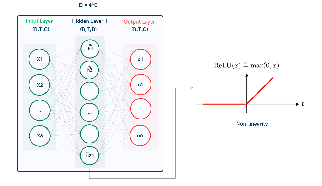
4.3 Feed-Forward Neural Network (FFNN)

The Feed-Forward Neural Network (FFNN) applies a pointwise transformation independently to each token's embedding dimension (much like in Linear Normalization) It processes each token vector through a small neural network comprising two linear layers separated by a non-linear activation function.

Input Dimensions: input $(B, T, C)$
First Linear Layer:
- Maps the input vectors ( $C$ -dimensional) to a higher-dimensional space ( $D = 4C$ ).
- The transformation is defined as: $$ \text{Output}_1 = X W_1 + b_1 $$
- $W_1$ : Weight matrix of shape $(C, D)$ .
- Resulting output: $(B, T, D)$ .
Non-Linear Activation:
- Applies a non-linear activation function (ReLU): $$ \text{Activated Output} = \text{ReLU}(\text{Output}_1) $$
Second Linear Layer:
- Reduces the dimensionality back to $C$ : $$ \text{Output}_2 = \text{Activated Output} W_2 + b_2 $$
- $W_2$ : Weight matrix of shape $(D, C)$ .
- Resulting output: $(B, T, C)$ .
Dropout:
- A dropout layer is applied to the output of the second linear layer to regularize the model and prevent overfitting.

Advantages of FFNN:

$D = 4C$ ensures the model captures richer, more complex representations.
Dropout improves generalization during training.

Example:

Input shape: $(B, T, C) = (1, 4, 6)$ .
The first linear layer (hidden) expands to $(1, 4, 4C) = (1, 4, 24)$ .
Apply ReLU activation.
The second linear layer reduces back to $(1, 4, C) = (1, 4, 6)$ .

When computing gradients during backpropagation, we go backward through the network, layer by layer, updating weights based on the gradient of the loss function. ReLU helps prevent gradients from vanishing by keeping gradients for positive inputs strong and setting gradients for inactive neurons (negative inputs) to zero, ensuring effective optimization. Basically, negative values don't contribute much, and small values lead to very small gradients (which slows learning).

4.4 Norm & Add (Pre-Norm)

After the Feed-Forward Neural Network (FFNN) step, the input undergoes the Norm & Add process, ensuring stability and efficient gradient flow through the network.

The output of the FFNN is added back to the input:

$\text{Output}_{\text{final}} = \text{Input} + \text{FFNN Output}$

This Norm & Add process ensures smooth training by stabilizing activations and maintaining efficient gradient flow.

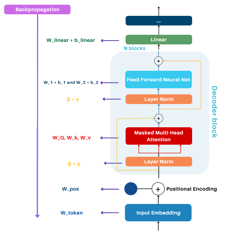
4.5. Full Decoder Block:

To build the full decoder-only Transformer block, we combine the following components:

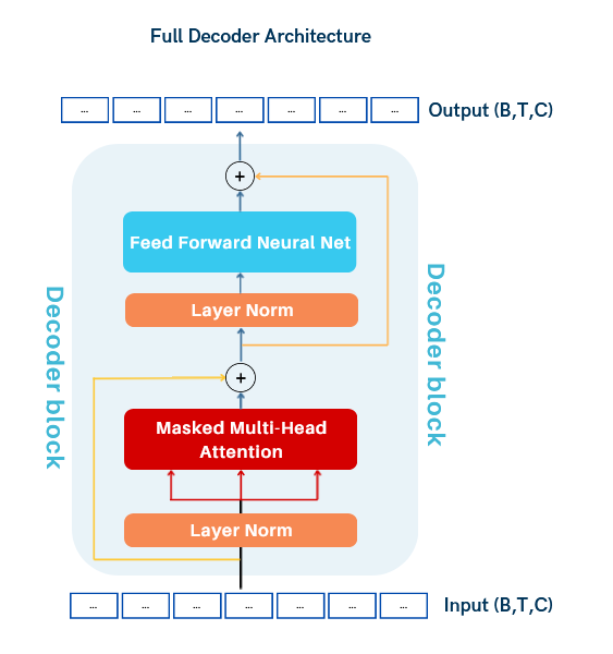
Masked Multi-Head Attention: Captures contextual relationships between tokens while respecting causality.
Norm and Add: Applies layer normalization and residual connection to stabilize training.
Feed-Forward Neural Network (FFNN): Introduces non-linear transformations to learn complex patterns.
Norm and Add: Another layer normalization and residual connection after the FFNN.

The input and output shapes remain the same ( $(B, T, C)$ ), but the model is now trained on sequences of batches, learning to process and generate sequences effectively.

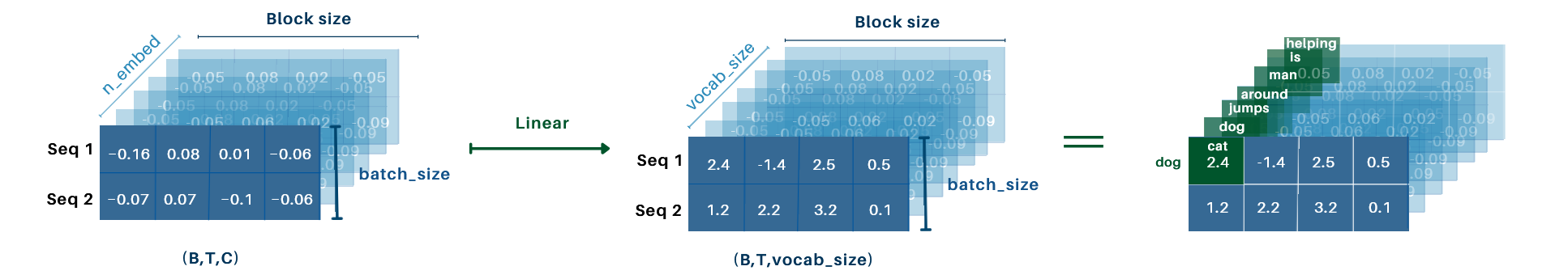
5. Linear Layer

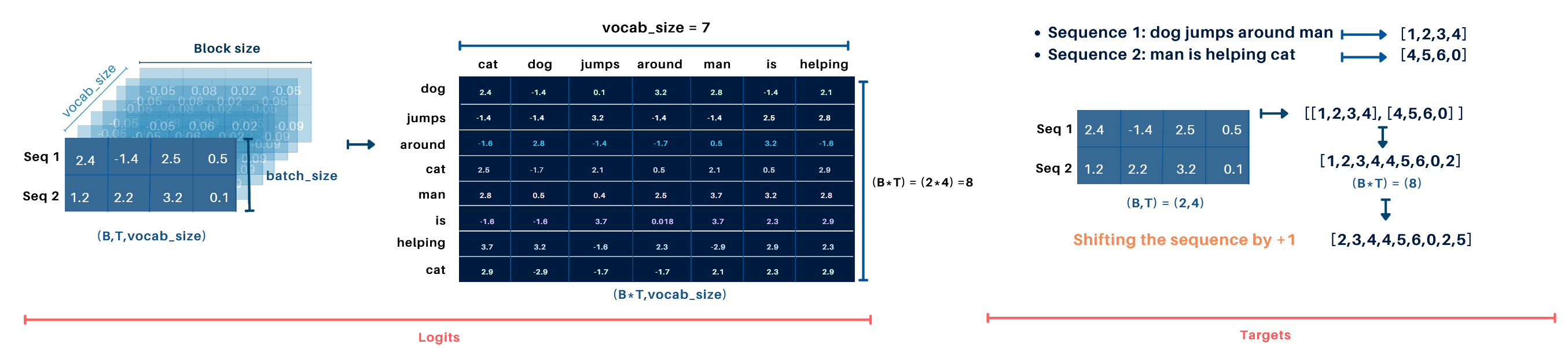
At the end of the decoder stack, the output is a tensor of shape $(B, T, C)$ This tensor needs to be mapped to logits over the vocabulary, which is achieved using the Linear Layer.

The Linear Layer projects the decoder output from shape $(B, T, C)$ to $(B, T, \text{vocab_size})$ .
Each element in the vocab_size dimension represents the raw score (logit) for a unique word in the vocabulary.

After the Linear Layer, the process differs depending on whether the model is in training or inference mode:

During Training: The logits are used to compute the loss by comparing predicted probabilities with the target labels.
During Inference: The logits are used to generate the next token

Example:

Input shape: $(B, T, C) = (2, 4, 6)$ .
Vocabulary size: $\text{vocab_size} = 7$ .
Output shape after the linear layer: $(B, T, \text{vocab_size}) = (2, 4, 7)$ .

For a sequence like "dog jumps around cat", each word in the sequence is mapped to every word in the vocabulary, providing unnormalized scores (logits) for all vocabulary words. For example:

First word "dog" produces unnormalized scores for all vocabulary words:
$\text{dog, cat}$ (logit: 2.3),
$\text{dog, dog}$ (logit: 4.1),
$\text{dog, jumps}$ (logit: 1.8),
$\text{dog, around}$ (logit: 3.0),
$\text{dog, man}$ (logit: 0.5),
$\text{dog, is}$ (logit: -1.2),
$\text{dog, helping}$ (logit: -0.8).

These unnormalized scores are the raw output of the final linear layer before applying softmax. This process is repeated for every token in the sequence.

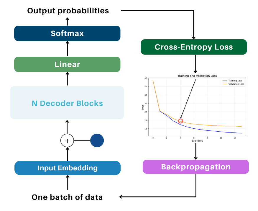
6. Training Pipeline

After the Linear Layer projects the decoder output to logits of shape $(B, T, \text{vocab_size})$ , the following steps occur during training*:

6.1. Flattening, Cross-Entropy Loss, Backpropagation

1. Flattening (with Target Shift by 1)

The logits are reshaped from $(B, T, \text{vocab_size})$ to $(B \cdot T, \text{vocab_size})$ , creating a 2D matrix suitable for loss computation.
The target labels, shifted by 1 to represent the next token, are flattened from $(B, T)$ to $(B \cdot T)$ , aligning with the logits.

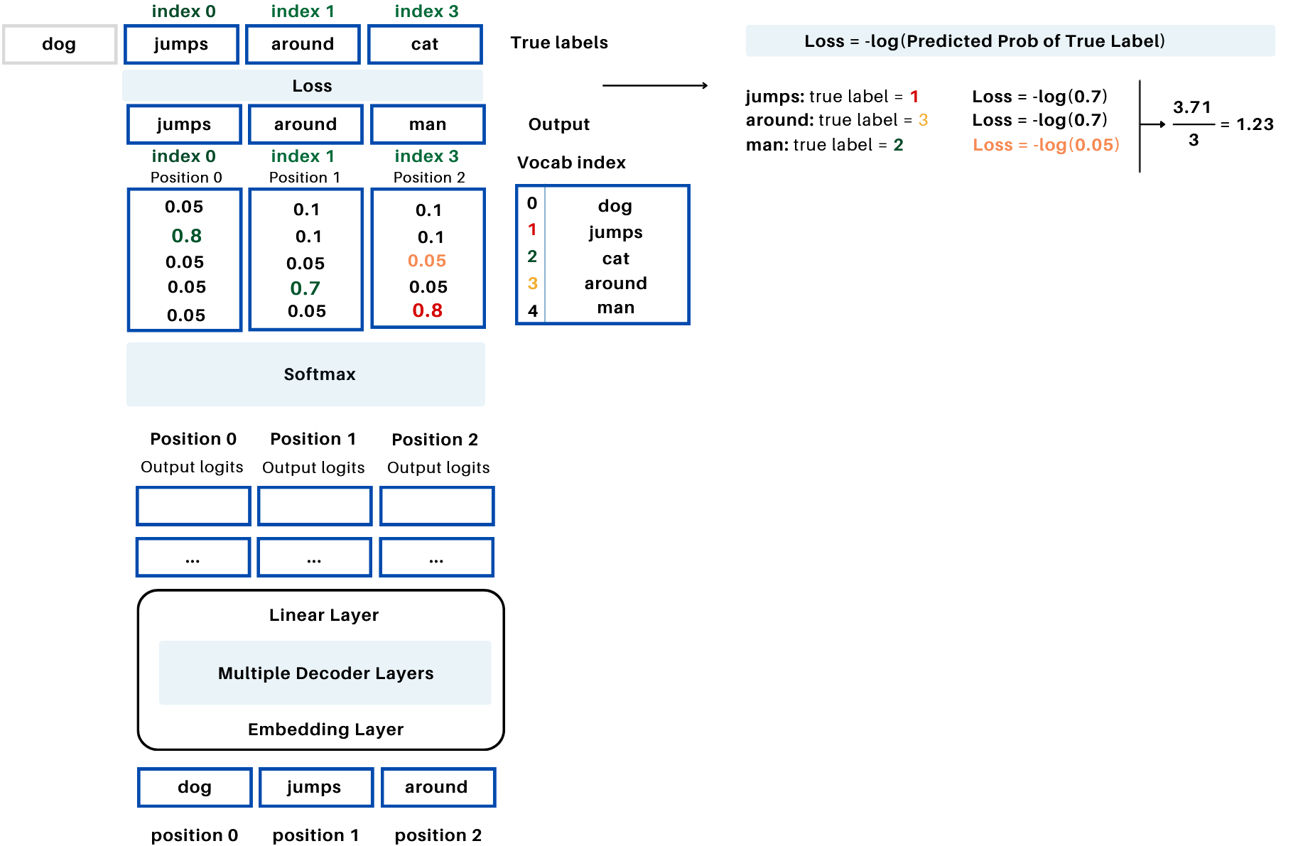
2. Cross-Entropy Loss

The Softmax function is applied to the logits to convert them into probabilities:

$P_i = \frac{\exp(\text{logit}_i)}{\sum_{j=1}^{\text{vocab_size}} \exp(\text{logit}_j)}$

$P_i$ is the probability of the $i$ -th token.
$\text{logit}_i$ is the logit (raw score) for the $i$ -th token.
The denominator sums the exponentials of all logits across the vocabulary

Note: In PyTorch, the Cross-Entropy Loss computes the softmax internally

The Cross-Entropy Loss is then computed as: $$ \text{Loss} = -\frac{1}{N} \sum_{i=1}^N \log P_{\text{target}_i} $$

$N = B \cdot T$ : Total number of tokens in the batch.
$P_{\text{target}_i}$ : Predicted probability of the target token.

Example:

3. Compute Gradients and Update Weights

Gradient Computation (Backpropagation): - During the forward pass, the model computes the loss. - Backpropagation calculates the gradients of the loss with respect to the model's weights: $$ \text{gradients} = \frac{\partial \text{Loss}}{\partial W} $$ - These gradients show how much each weight contributes to the loss. - The gradients are stored in the .grad attribute of each weight.

Weight Update (Optimizer): - Using the computed gradients, the optimizer updates the model's weights. - The optimizer applies the update rule (e.g., for Adam or SGD): $$ W_{\text{new}} = W_{\text{old}} - \eta \cdot \frac{\partial \text{Loss}}{\partial W} $$ - $W_{\text{new}}$ : Updated weight.
- $W_{\text{old}}$ : Current weight.
- $\eta$ : Learning rate.

6.2. Learnable Weights Update

Embedding Weights:
- Token Embedding Table: Maps tokens to embeddings.
- Positional Embedding Table: Provides positional encodings.
Attention Weights:
- Query, Key, Value Weight Matrices: $W_Q, W_K, W_V$ for attention computation.
- Final Projection Matrix: Aggregates multi-head attention outputs.
FFNN Weights:
- First Linear Layer: Weights $W_1$ and bias $b_1$ .
- Second Linear Layer: Weights $W_2$ and bias $b_2$ .
Layer Normalization Weights:
- Scaling parameter: $\gamma$ .
- Shifting parameter: $\beta$ .
Linear Layer Weights:
- Weight matrix and bias used in the final projection to logits.

Note: The optimizer updates all these weights during the optimization step, using the gradients computed via backpropagation.

6.3. Loss Computation During Training

During training, the loss is computed for the entire batch by aggregating the errors across all tokens in all sequences within the batch and averaging them. This single loss value represents the overall error for the batch. The loss is then used to update the model's weights through backpropagation, optimizing the network to minimize future errors.

To monitor performance, the loss on validation data is also computed periodically (e.g., after a certain number of iterations). During this step, the model is set to evaluation mode (using model.eval()) to ensure that weights are not modified and that behaviors like dropout are disabled. This helps assess how well the model generalizes to unseen data without impacting the training process.

7. Inference Pipeline

In generation mode, the model predicts one token at a time, iteratively building the output sequence using weights and embeddings learned during training, which allows the model to generate coherent and context-aware text outputs.

7.1. Input Preparation

User Input:The process begins with an input sequence or prompt (e.g., "dog").
Tokenization, Embedding, Positional Encodings:
- The input is tokenized and mapped to token indices.
- These indices are passed through the learned embedding matrix to produce an embedding tensor of shape (B,T,C)
- Positional encodings (learned during training) are added to the token embeddings.

7.2. Autoregressive Token Prediction

Passing Through the Model:The input tensor $(B, T, C)$ is passed through the model's decoder, using weights and parameters learned during training.
Decoder Components:
- Masked Multi-Head Attention: Computes attention over past tokens only, ensuring causality.
- Feed-Forward Neural Network (FFNN): Applies non-linear transformations to enrich token representations.
- Final Linear Layer: Maps the decoder output to logits (B,T,vocab_size)
Softmax and Token Selection:
- The logits are passed through a softmax function to compute probabilities over the vocabulary.
- The token with the highest probability (or sampling) is chosen as the next token.

7.3. Iterative Process

Token Appending: The newly predicted token is appended to the input sequence, which grows in length: (B,T+1,C)
Iteration: the process repeats until a stopping condition is met, such as reaching the maximum number of new tokens.

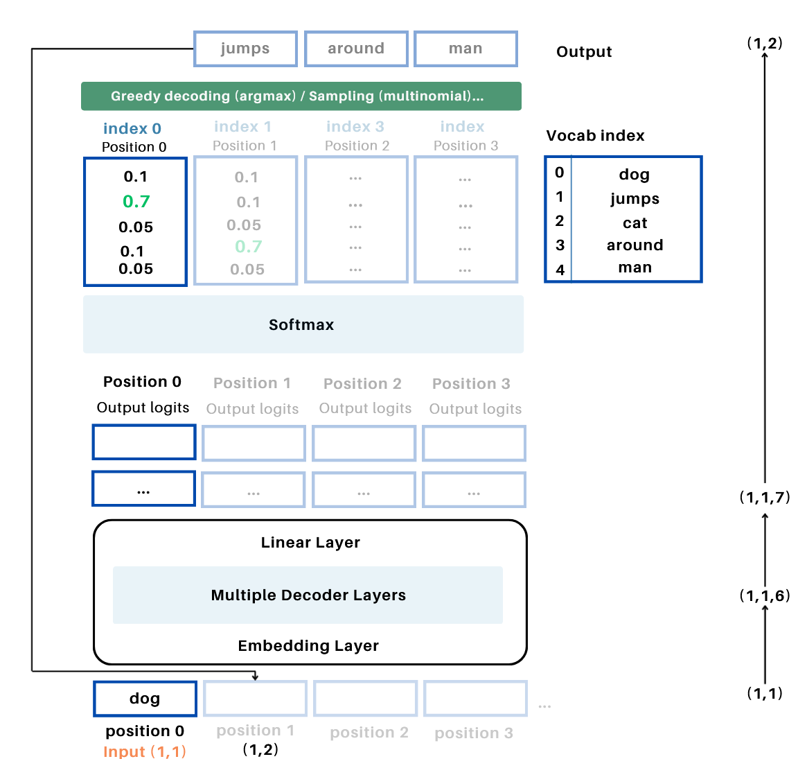
Example: Iterative Token Generation

Initial Input:
- Start with the input sequence, e.g., "dog" (token at position 0).
- After tokenization and embedding, the input shape is $(B=1, T=1, C)$ , where $C$ is the embedding dimension.
First Iteration:
- Pass the input tensor $(1, 1, C)$ through the model.
- The model generates logits for position 1 with shape $(1, 1, \text{vocab_size})$ .
- Apply softmax to the logits to compute probabilities over the vocabulary.
- Use argmax or a sampling strategy to select the next token, e.g., "jumps" (index 1).
- Update: Append "jumps" to the sequence. The input tensor updates to $(1, 2)$ , and then transformed to (1,2,C) when fed to the model.
Second Iteration:
- Pass the updated sequence ("dog", "jumps") with shape $(1, 2, C)$ through the model.
- The model generates logits for position 2 with shape $(1, 2, \text{vocab_size})$ .
- Apply softmax, then argmax to select the next token, e.g., "around" (index 3).
- Update: Append "around" to the sequence. The input tensor updates to $(1, 3, C)$ .
Repeat:
- Continue passing the updated sequence through the model, generating logits for the next position, and appending the predicted token.
- The process continues until a stopping criterion is met, such as reaching a predefined sequence length.

10. Additionals: Vanishing Gradients, Exploding Gradients, and Regularization Techniques

Gradients, computed during backpropagation, are the derivatives of the loss function with respect to model parameters (weights). They guide how much each parameter should change to minimize the loss. However, gradients can sometimes vanish or explode, causing training difficulties and poor model performance.

Vanishing Gradients: Gradients become very small as they propagate backward through the network, especially with activation functions like sigmoid or tanh. These functions saturate at high or low input values, producing near-zero gradients. Additionally, weights $W < 1$ during backpropagation shrink gradients exponentially, causing training to stall.
Exploding Gradients: Conversely, gradients can grow excessively large ( $W > 1$ ), leading to unstable training and erratic weight updates.

To stabilize training and improve gradient flow, several techniques are commonly used:

Weight Initialization: Proper initialization methods, like Xavier or He initialization, ensure gradients neither vanish nor explode during forward and backward passes.
Activation Functions: ReLU avoids saturation by zeroing out negative values and maintaining constant gradients ( $f'(x) = 1$ ) for positive values. Variants like Leaky ReLU further improve gradient flow.
Gradient Clipping: Limits the magnitude of gradients to a predefined threshold, preventing exploding gradients by capping excessively large values.
Normalization Techniques:
- Layer Normalization stabilizes gradient flow by standardizing activations, helping to prevent both vanishing and exploding gradients.
- Batch Normalization reduces internal covariate shift, improving gradient stability.
Regularization Techniques:
- Dropout: Randomly drops neurons during training, improving robustness and stabilizing gradient reliance.
- Weight Decay: Penalizes large weights, mitigating exploding gradients.
- Learning Rate Schedulers: Gradually reduce the learning rate during training, ensuring smoother weight updates.
Optimizers: Advanced optimizers like Adam adapt learning rates for each parameter, stabilizing gradient updates and improving convergence.

Decoder-Only Transformer Architecture

Table of Contents

1. Introduction

2. Architecture Overview

3. Input Tokens, Embedding, and Positional Encoding

Example:

4. Decoder:

4.1. Masked Multi-Head Attention

Example:

4.2. Norm & Add (Pre-norm)

4.3 Feed-Forward Neural Network (FFNN)

Example:

4.4 Norm & Add (Pre-Norm)

4.5. Full Decoder Block:

5. Linear Layer

Example:

6. Training Pipeline

6.1. Flattening, Cross-Entropy Loss, Backpropagation

Example:

6.2. Learnable Weights Update

6.3. Loss Computation During Training

7. Inference Pipeline

7.1. Input Preparation

7.2. Autoregressive Token Prediction

7.3. Iterative Process

Example: Iterative Token Generation

10. Additionals: Vanishing Gradients, Exploding Gradients, and Regularization Techniques

8. References: